Examples
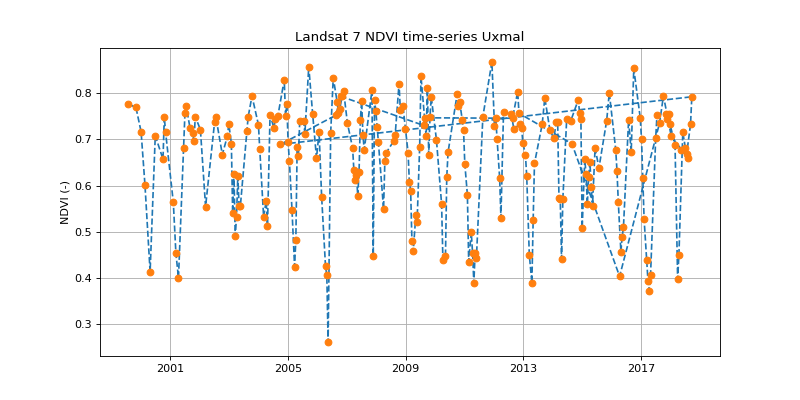
First example: extract a time-series using the API and plot it with matplotlib
from geextract import ts_extract, get_date
from datetime import datetime
import numpy as np
import matplotlib.pyplot as plt
plt.figure(figsize=(10,5))

# Extract a Landsat 7 time-series for a 500m radius circular buffer around
# a location in Yucatan
lon = -89.8107197
lat = 20.4159611
raw_dict = ts_extract(lon=lon, lat=lat, sensor='LE7',
                      start=datetime(1999, 1, 1), radius=500)

# Function to compute ndvi from a dictionary of the list of dictionaries returned
# by ts_extract
def ndvi(x):
    try:
        return (x['B4'] - x['B3']) / (x['B4'] + x['B3'])
    except:
        pass

# Build x and y arrays and remove missing values
x = np.array([get_date(d['id']) for d in raw_dict])
y = np.array([ndvi(d) for d in raw_dict], dtype=np.float)
x = x[~np.isnan(y)]
y = y[~np.isnan(y)]

# Make plot
plt.plot_date(x, y, "--")
plt.plot_date(x, y)
plt.title("Landsat 7 NDVI time-series Uxmal")
plt.ylabel("NDVI (-)")
plt.grid(True)
plt.show()
(Source code, png, hires.png, pdf)

Second example: extract a time-series using the command line and read it in R
gee_extract.py -s LT5 -b 1980-01-01 -lon -89.8107 -lat 20.4159 -r 500 -db /tmp/gee_db.sqlite -site uxmal -table col_1
gee_extract.py -s LE7 -b 1980-01-01 -lon -89.8107 -lat 20.4159 -r 500 -db /tmp/gee_db.sqlite -site uxmal -table col_1
gee_extract.py -s LC8 -b 1980-01-01 -lon -89.8107 -lat 20.4159 -r 500 -db /tmp/gee_db.sqlite -site uxmal -table col_1
Running the three above commands gives you the following terminal output. Records refer to individual time steps at which Landsat observations were extracted. Note that some records may be “empty” due to absence of useful data after the cloud masking step. The amount of useful data of the entire time-series is therefore likely to be less than the reported extracted records.
Extracted 148 records from Google Eath Engine
Extracted 231 records from Google Eath Engine
Extracted 82 records from Google Eath Engine
A sqlite database has been created at /tmp/gee_db.sqlite; it contains a table named col_1 (for “collection 1”) that can be read as an R dataframe using tools like dplyr.
library(dplyr)
library(DBI)

# Open database connection (requires dbplyr and RSQLite packages, DBI installed via dbplyr)
con <- dbConnect(RSQLite::SQLite(), dbname = "/tmp/gee_db.sqlite")
dbListTables(con)
df <- tbl(con, 'col_1') %>% collect()
df
In that case the table contains only one time-series (uxmal site); we are therefore loading the whole table in memory using collect() without additional filtering query.
[1] "col_1"

# A tibble: 390 x 11
   index  blue green id                     nir   red swir1 swir2 time       sensor site
   <int> <dbl> <dbl> <chr>                <dbl> <dbl> <dbl> <dbl> <chr>      <chr>  <chr>
 1     0   434   635 LT05_020046_19850206  2077   675  2267  1281 1985-02-06 LT5    uxmal
 2     1   370   664 LT05_020046_19850427  2883   588  2136  1128 1985-04-27 LT5    uxmal
 3     2   385   592 LT05_020046_19860108  2732   553  2010   953 1986-01-08 LT5    uxmal
 4     3   555   748 LT05_020046_19860313  1971   823  2497  1479 1986-03-13 LT5    uxmal
 5     4   574   804 LT05_020046_19860414  2216   919  2751  1701 1986-04-14 LT5    uxmal
 6     5   790  1084 LT05_020046_19860703  3852   955  2205  1121 1986-07-03 LT5    uxmal
 7     6   546   858 LT05_020046_19860820  3876   730  1968   896 1986-08-20 LT5    uxmal
 8     7   334   560 LT05_020046_19861007  2694   532  2088  1072 1986-10-07 LT5    uxmal
 9     8   321   539 LT05_020046_19861023  2550   524  2064  1082 1986-10-23 LT5    uxmal
10     9   590   832 LT05_020046_19870417  2390   891  2752  1660 1987-04-17 LT5    uxmal
# ... with 380 more rows
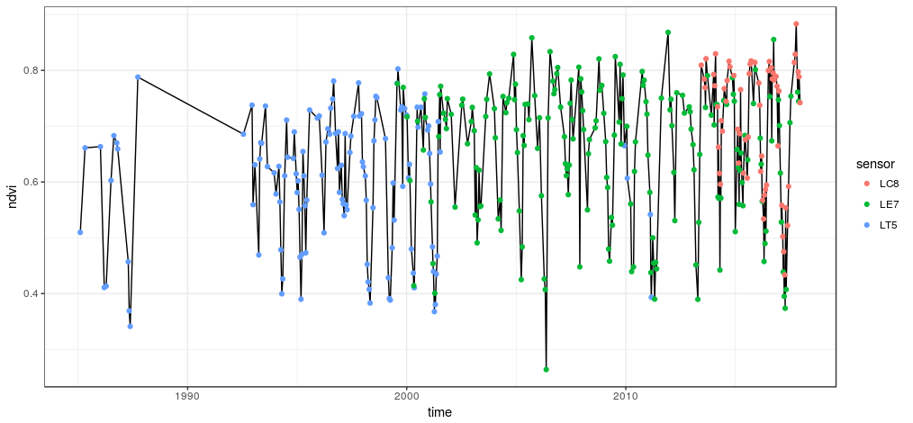
This dataframe (or tibble) can now be used as the base for all kind of data analysis in R. Here we’ll make some simple plots using the ggplot2 package.
library(ggplot2)
library(tidyr)

df %>% mutate(ndvi = (nir - red) / (nir + red)) %>%
  ggplot(aes(time, ndvi)) +
    geom_line() +
    geom_point(aes(col = sensor)) +
    theme_bw()
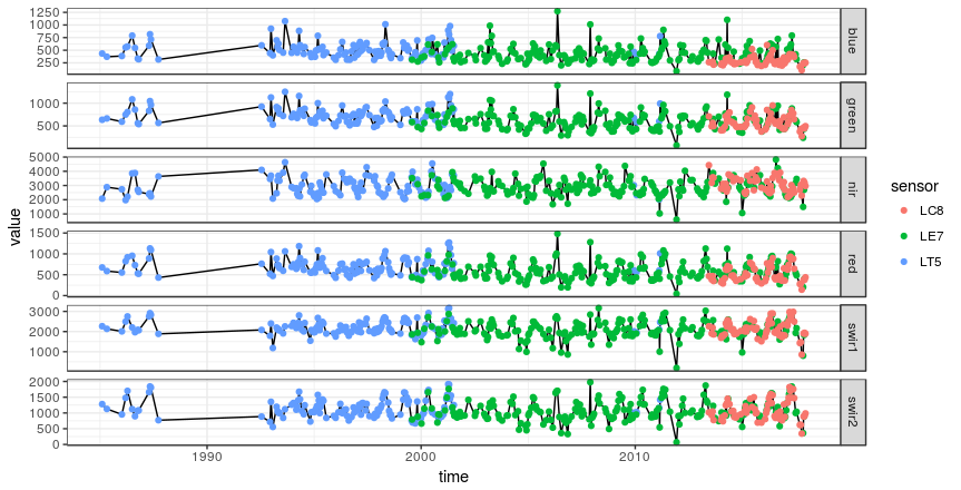
df %>% gather(key, value, -c(time, index, sensor, site, id)) %>%
  ggplot(aes(time, value)) +
    geom_line() +
    geom_point(aes(col = sensor)) +
    facet_grid(key ~ ., scales = 'free') +
    theme_bw()
The idea when working with multiple sites is to append them all to the same database table and use sql (raw or via dplyr) to filter the desired data. Ordering time-series for multiple sites can be done in batch thanks to the gee_extract_batch.py command (run gee_extract_batch.py --help to see the detailed usage instructions). Here we will simply append another site to the sqlite table by re-running the gee_extract.py commands with different coordinates.
gee_extract.py -s LT5 -b 1980-01-01 -lon 4.7174 -lat 44.7814 -r 500 -db /tmp/gee_db.sqlite -site rompon -table col_1
gee_extract.py -s LE7 -b 1980-01-01 -lon 4.7174 -lat 44.7814 -r 500 -db /tmp/gee_db.sqlite -site rompon -table col_1
gee_extract.py -s LC8 -b 1980-01-01 -lon 4.7174 -lat 44.7814 -r 500 -db /tmp/gee_db.sqlite -site rompon -table col_1
Extracted 104 records from Google Eath Engine
Extracted 494 records from Google Eath Engine
Extracted 193 records from Google Eath Engine
Now the col_1 sqlite table contains time-series for two different sites (uxmal and rompon). Loading the time-series of a single site can be done thanks to the filter() dplyr verb.
df <- tbl(con, 'col_1') %>%
  filter(site == 'rompon') %>%
  collect() %>%
  mutate(time = as.Date(time))
df
# A tibble: 513 x 11
   index  blue green id                     nir   red swir1 swir2 time       sensor site
   <int> <dbl> <dbl> <chr>                <dbl> <dbl> <dbl> <dbl> <date>     <chr>  <chr>
 1     0  1023  1179 LT05_196029_19840409  2438  1193  2096  1329 1984-04-09 LT5    rompon
 2     1   822  1035 LT05_196029_19840425  2561   987  2025  1125 1984-04-25 LT5    rompon
 3     4   451   715 LT05_196029_19840612  3481   582  1893   870 1984-06-12 LT5    rompon
 4     6   481   691 LT05_196029_19840815  2935   624  1799   866 1984-08-15 LT5    rompon
 5     7   370   590 LT05_196029_19840831  2880   534  1736   818 1984-08-31 LT5    rompon
 6     8   358   580 LT05_196029_19841002  2833   510  1560   708 1984-10-02 LT5    rompon
 7    10   408   642 LT05_196029_19841119  2491   656  1693   817 1984-11-19 LT5    rompon
 8    13   744   991 LT05_196029_19850327  2284  1033  2046  1239 1985-03-27 LT5    rompon
 9    16   579   845 LT05_196029_19850530  3678   697  2114   999 1985-05-30 LT5    rompon
10    17   546   800 LT05_196029_19850615  3697   654  1928   933 1985-06-15 LT5    rompon
# ... with 503 more rows
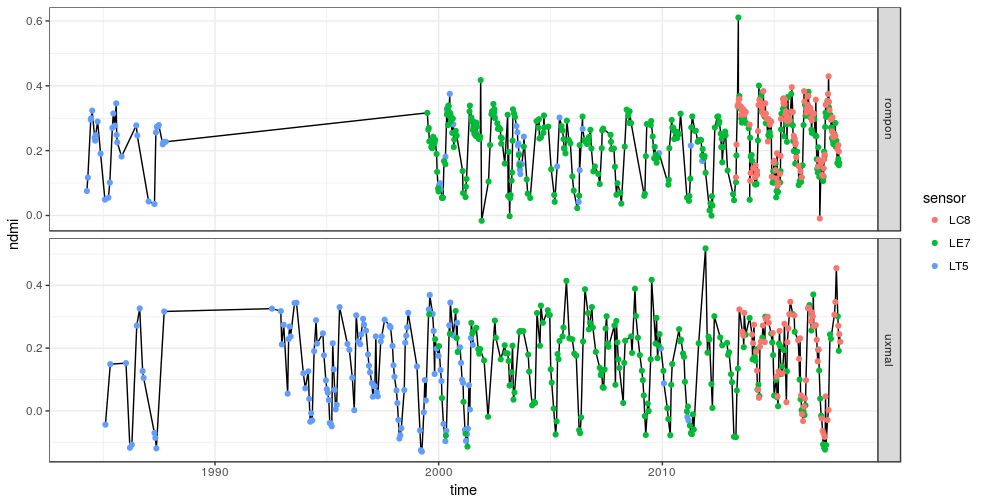
It is also possible to load the entire table to for instance plot the two time-series side by side.
df <- tbl(con, 'col_1') %>%
  collect() %>%
  mutate(time = as.Date(time))

df %>% mutate(ndmi = (nir - swir1) / (nir + swir1)) %>%
    ggplot(aes(time, ndmi)) +
      geom_line() +
      geom_point(aes(col = sensor)) +
      facet_grid(site ~ ., scales = 'free') +
      theme_bw()
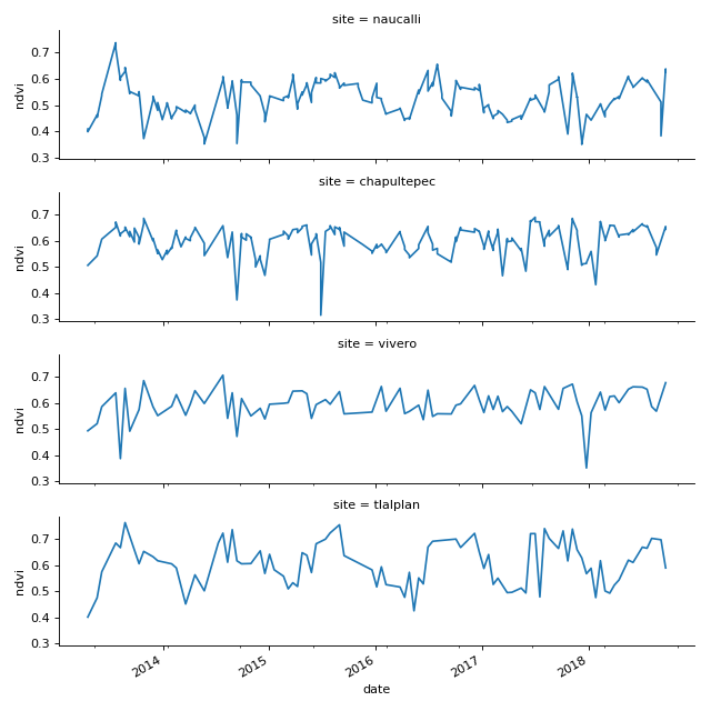
Third example: Extract time-series for each feature of a polygon feature collection
The file cdmx_parks.gpkg contains contours of some of the parks of Mexico City. The example below extracts the spatially aggregated time-series for each of these parks, writes the results to a sqlite database and reads the data back into python for plotting.
from geextract import ts_extract, relabel, date_append, dictlist2sqlite
import fiona
import pandas as pd
import seaborn as sns
import matplotlib.pyplot as plt

import sqlite3
from datetime import datetime
import os

try:
    os.remove('/tmp/landsat_cdmx.sqlite')
except:
    pass

# Open feature collection generator
with fiona.open('data/cdmx_parks.gpkg', layer='parks') as src:
    # Iterate over feature collection
    for feature in src:
        # Extract time-series
        ts_0 = ts_extract(sensor='LC8', start=datetime(2012, 1, 1),
                          feature=feature)
        ts_1 = relabel(ts_0, 'LC8')
        ts_2 = date_append(ts_1)
        # Write dictionnary list to sqlite database table
        dictlist2sqlite(ts_2, site=feature['properties']['name'],
                        sensor='LC8', db_src='/tmp/landsat_cdmx.sqlite',
                        table='cdmx')

# REad the data back into a pandas dataframe
conn = sqlite3.connect("/tmp/landsat_cdmx.sqlite")
df = pd.read_sql_query('select * from cdmx', conn)
df['date'] = pd.to_datetime(df['time'], format='%Y-%m-%d')
df['ndvi'] = (df.nir - df.red) / (df.nir + df.red)
# Make facetgrid plot
g = sns.FacetGrid(df, row='site', aspect=4, size=2)
def dateplot(x, y, **kwargs):
    ax = plt.gca()
    data = kwargs.pop("data")
    data.plot(x=x, y=y, ax=ax, grid=False, **kwargs)
g = g.map_dataframe(dateplot, "date", "ndvi")
plt.show()
(Source code, png, hires.png, pdf)
